甲乙小朋友的房子

甲乙小朋友很笨,但甲乙小朋友不会放弃

0%

深度学习实践-1-3-构建浅层神经网络

序言

本文主要参考自吴恩达Coursera深度学习课程 DeepLearning.ai 编程作业(1-3)

吴恩达Coursera课程 DeepLearning.ai 编程作业系列,本文为《神经网络与深度学习》部分的第三周“浅层神经网络”的课程作业。

本节的主要内容是:利用浅层神经网络实现平面数据分类

1 - import的包

  • numpy
  • sklearn
  • matplotlib
  • testCase - 提供了测试样例
  • pannar_utils - 一些有用的工具
1
2
3
4
5
6
7
8
9
10
11
12
13
14
15
import warnings
warnings.filterwarnings("ignore")

# Package imports
import numpy as np
import matplotlib.pyplot as plt
from testCases import *
import sklearn
import sklearn.datasets
import sklearn.linear_model
from planar_utils import plot_decision_boundary, sigmoid, load_planar_dataset, load_extra_datasets

%matplotlib inline

np.random.seed(1) # 给np.random设定一个种子,这样随机数就固定了

2 - 数据集

下面的代码生成了“花”的二类数据集

1
2
3
4
5
6
7
8
9
10
11
12
13
14
15
16
17
18
19
20
21
22
23
24
25
# 这个函数原本在panar_utils.py里
def load_planar_dataset():
np.random.seed(1)
m = 400 # 样本数量
N = int(m/2) # 每个类别的数量
D = 2 # 维度
# 初始化X,Y
X = np.zeros((m,D))
Y = np.zeros((m,1),dtype='uint8')
a = 4 # 花儿最大长度

for j in range(2):
ix = range(N*j,N*(j+1))
t = np.linspace(j*3.12,(j+1)*3.12,N) + np.random.randn(N)*0.2 # theta
r = a*np.sin(4*t) + np.random.randn(N)*0.2 # radius
X[ix] = np.c_[r*np.sin(t), r*np.cos(t)]
Y[ix] = j

X = X.T
Y = Y.T

return X, Y

X,Y = load_planar_dataset()
print X.shape,Y.shape
(2L, 400L) (1L, 400L)

此时你得到了:

  • 一个numpy-array(matrix) X,包括特征(X1,X2)
  • 一个numpy-arrya(vector) Y,包含一列标签(0或1)

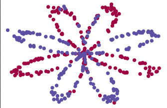
接下来用matplotlib将这个“花儿”数据集可视化,其中: - y = 0 -> 红色 - y = 1 -> 蓝色

我们的目标是建立一个模型,能将红色和蓝色分开

1
2
# 数据可视化
plt.scatter(X[0, :], X[1, :], c=Y, s=40, cmap=plt.cm.Spectral)

简单的逻辑回归

首先我们看看LR在这个问题上表现如何:

1
2
3
4
5
6
7
8
9
10
11
12
# Train the logistic regression classifier
clf = sklearn.linear_model.LogisticRegressionCV();
clf.fit(X.T, Y.T);

# 画出LR的决策边界
plot_decision_boundary(lambda x: clf.predict(x), X, Y)
plt.title("Logistic Regression")

# 打印准确率
LR_predictions = clf.predict(X.T)
print ('LR的准确率是: %d ' % float((np.dot(Y,LR_predictions) + np.dot(1-Y,1-LR_predictions))/float(Y.size)*100) +
'% ')
LR的准确率是: 47 % 

1
2
3
4
5
6
7
8
9
10
11
12
13
14
15
16
17
# 以上的plot_decision_boundary()函数定义如下:

def plot_decision_boundary(model, X, y):
# Set min and max values and give it some padding
x_min, x_max = X[0, :].min() - 1, X[0, :].max() + 1
y_min, y_max = X[1, :].min() - 1, X[1, :].max() + 1
h = 0.01
# Generate a grid of points with distance h between them
xx, yy = np.meshgrid(np.arange(x_min, x_max, h), np.arange(y_min, y_max, h))
# Predict the function value for the whole grid
Z = model(np.c_[xx.ravel(), yy.ravel()])
Z = Z.reshape(xx.shape)
# Plot the contour and training examples
plt.contourf(xx, yy, Z, cmap=plt.cm.Spectral)
plt.ylabel('x2')
plt.xlabel('x1')
plt.scatter(X[0, :], X[1, :], c=y, cmap=plt.cm.Spectral)
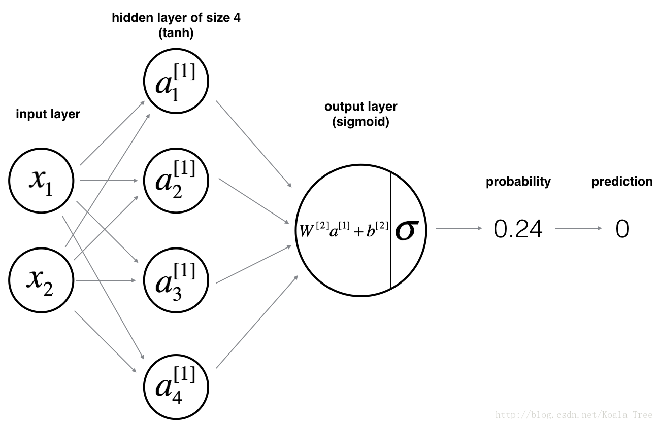
神经网络模型

我们本次模型为:

数学模型 对于一条样本\(x^{i}\)

\[z^{[1] (i)} = W^{[1]} x^{(i)} + b^{[1] (i)}\tag{1}\] \[a^{[1] (i)} = \tanh(z^{[1] (i)})\tag{2}\] \[z^{[2] (i)} = W^{[2]} a^{[1] (i)} + b^{[2] (i)}\tag{3}\] \[\hat{y}^{(i)} = a^{[2] (i)} = \sigma(z^{ [2] (i)})\tag{4}\] \[y^{(i)}_{prediction} = \begin{cases} 1 & \mbox{if } a^{[2](i)} > 0.5 \\ 0 & \mbox{otherwise } \end{cases}\tag{5}\]

通过上式计算出所有样本的预测误差,我们可以通过下式计算出误差函数: \[J = - \frac{1}{m} \sum\limits_{i = 0}^{m} \large\left(\small y^{(i)}\log\left(a^{[2] (i)}\right) + (1-y^{(i)})\log\left(1- a^{[2] (i)}\right) \large \right) \small \tag{6}\]

回忆一下,计算神经网络的步骤为: 1. 定义网络结构 2. 初始化模型参数 3. 迭代 - 前向传播计算预测值 - 计算误差 - 后向传播计算梯度 - 根据梯度更新参数

定义网络结构

约定: - n_x : 输入层的数据个数 - n_h : 隐藏层数 (此处设置为4) - n_y : 输出层的数据个数(类别个数)

可定义如下函数来获取以上三个数

1
2
3
4
5
6
7
8
9
10
11
12
13
14
15
16
17
18
19
20
21
22
23
24
# GRADED FUNCTION: layer_sizes

def layer_sizes(X, Y):
"""
Arguments:
X -- input dataset of shape (input size, number of examples)
Y -- labels of shape (output size, number of examples)

Returns:
n_x -- the size of the input layer
n_h -- the size of the hidden layer
n_y -- the size of the output layer
"""
### START CODE HERE ### (≈ 3 lines of code)
n_x = X.shape[0] # size of input layer
n_h = 4
n_y = Y.shape[0]# size of output layer
### END CODE HERE ###
return (n_x, n_h, n_y)
n_x, n_h, n_y = layer_sizes(X,Y)

print "n_x = ",n_x
print "n_h = ",n_h
print "n_y = ",n_y
n_x =  2
n_h =  4
n_y =  1

初始化参数

需要初始化的参数主要是W和b

Exercise: Implement the function initialize_parameters().

Instructions: - Make sure your parameters’ sizes are right. Refer to the neural network figure above if needed. - You will initialize the weights matrices with random values. - Use: np.random.randn(a,b) * 0.01 to randomly initialize a matrix of shape (a,b). - You will initialize the bias vectors as zeros. - Use: np.zeros((a,b)) to initialize a matrix of shape (a,b) with zeros.

1
2
3
4
5
6
7
8
9
10
11
12
13
14
15
16
17
18
19
20
21
22
23
24
25
26
27
28
29
30
31
32
33
34
35
36
37
38
39
40
41
42
43
# GRADED FUNCTION: initialize_parameters

def initialize_parameters(n_x, n_h, n_y):
"""
Argument:
n_x -- size of the input layer
n_h -- size of the hidden layer
n_y -- size of the output layer

Returns:
params -- python dictionary containing your parameters:
W1 -- weight matrix of shape (n_h, n_x)
b1 -- bias vector of shape (n_h, 1)
W2 -- weight matrix of shape (n_y, n_h)
b2 -- bias vector of shape (n_y, 1)
"""

np.random.seed(2) # we set up a seed so that your output matches ours although the initialization is random.

### START CODE HERE ### (≈ 4 lines of code)
W1 = np.random.randn(n_h, n_x)
b1 = np.zeros((n_h, 1))
W2 = np.random.randn(n_y, n_h)
b2 = np.zeros((n_y, 1))
### END CODE HERE ###

assert (W1.shape == (n_h, n_x))
assert (b1.shape == (n_h, 1))
assert (W2.shape == (n_y, n_h))
assert (b2.shape == (n_y, 1))

parameters = {"W1": W1,
"b1": b1,
"W2": W2,
"b2": b2}

return parameters

parameters = initialize_parameters(n_x, n_h, n_y)
print("W1 = " + str(parameters["W1"]))
print("b1 = " + str(parameters["b1"]))
print("W2 = " + str(parameters["W2"]))
print("b2 = " + str(parameters["b2"]))
W1 = [[-0.41675785 -0.05626683]
 [-2.1361961   1.64027081]
 [-1.79343559 -0.84174737]
 [ 0.50288142 -1.24528809]]
b1 = [[ 0.]
 [ 0.]
 [ 0.]
 [ 0.]]
W2 = [[-1.05795222 -0.90900761  0.55145404  2.29220801]]
b2 = [[ 0.]]

迭代

前向传播

问题: 实现 forward_propagation().

Instructions: - Look above at the mathematical representation of your classifier. - You can use the function sigmoid(). It is built-in (imported) in the notebook. - You can use the function np.tanh(). It is part of the numpy library. - The steps you have to implement are: 1. Retrieve each parameter from the dictionary "parameters" (which is the output of initialize_parameters()) by using parameters[".."]. 2. Implement Forward Propagation. Compute \(Z^{[1]}, A^{[1]}, Z^{[2]}\) and \(A^{[2]}\) (the vector of all your predictions on all the examples in the training set). - Values needed in the backpropagation are stored in "cache". The cache will be given as an input to the backpropagation function.

1
2
3
4
5
6
7
8
9
10
11
12
13
14
15
16
17
18
19
20
21
22
23
24
25
26
27
28
29
30
31
32
33
34
35
36
37
38
39
40
41
42
43
44
# 前向传播

def forward_propagation(X, parameters):
"""
Argument:
X -- input data of size (n_x, m)
parameters -- python dictionary containing your parameters (output of initialization function)

Returns:
A2 -- The sigmoid output of the second activation
cache -- a dictionary containing "Z1", "A1", "Z2" and "A2"
"""
# Retrieve each parameter from the dictionary "parameters"
### START CODE HERE ### (≈ 4 lines of code)
# 参数获取
W1 = parameters["W1"]
b1 = parameters["b1"]
W2 = parameters["W2"]
b2 = parameters["b2"]
### END CODE HERE ###

# Implement Forward Propagation to calculate A2 (probabilities)
### START CODE HERE ### (≈ 4 lines of code)
# 计算预测值
Z1 = np.dot(W1, X) + b1
A1 = np.tanh(Z1)
Z2 = np.dot(W2, A1) + b2
A2 = sigmoid(Z2)
### END CODE HERE ###

assert(A2.shape == (1, X.shape[1]))

cache = {"Z1": Z1,
"A1": A1,
"Z2": Z2,
"A2": A2}

return A2, cache

X_assess, parameters = forward_propagation_test_case()
A2, cache = forward_propagation(X_assess, parameters)

# Note: we use the mean here just to make sure that your output matches ours.
print(np.mean(cache['Z1']) ,np.mean(cache['A1']),np.mean(cache['Z2']),np.mean(cache['A2']))
(-0.00049975577774199022, -0.00049696335323177901, 0.00043818745095914658, 0.50010954685243103)

计算误差

现在我们已经计算除了预测值A2,接下来我们需要计算本轮误差:

\[J = - \frac{1}{m} \sum\limits_{i = 0}^{m} \large{(} \small y^{(i)}\log\left(a^{[2] (i)}\right) + (1-y^{(i)})\log\left(1- a^{[2] (i)}\right) \large{)} \small\tag{13}\]

Exercise: Implement compute_cost() to compute the value of the cost \(J\).

Instructions: - There are many ways to implement the cross-entropy loss. To help you, we give you how we would have implemented \(- \sum\limits_{i=0}^{m} y^{(i)}\log(a^{[2](i)})\):

1
2
logprobs = np.multiply(np.log(A2),Y)
cost = - np.sum(logprobs) # no need to use a for loop!

(you can use either np.multiply() and then np.sum() or directly np.dot()).

1
2
3
4
5
6
7
8
9
10
11
12
13
14
15
16
17
18
19
20
21
22
23
24
25
26
27
28
29
30
31
32
# GRADED FUNCTION: compute_cost

def compute_cost(A2, Y, parameters):
"""
Computes the cross-entropy cost given in equation (13)

Arguments:
A2 -- The sigmoid output of the second activation, of shape (1, number of examples)
Y -- "true" labels vector of shape (1, number of examples)
parameters -- python dictionary containing your parameters W1, b1, W2 and b2

Returns:
cost -- cross-entropy cost given equation (13)
"""

m = Y.shape[1] # number of example

# Compute the cross-entropy cost
### START CODE HERE ### (≈ 2 lines of code)
# 误差计算
logprobs = np.multiply(np.log(A2), Y) + np.multiply(np.log(1-A2), (1-Y))
cost = -(1.0/m)*np.sum(logprobs)
### END CODE HERE ###

cost = np.squeeze(cost) # makes sure cost is the dimension we expect.
# E.g., turns [[17]] into 17
assert(isinstance(cost, float))

return cost
A2, Y_assess, parameters = compute_cost_test_case()

print("cost = " + str(compute_cost(A2, Y_assess, parameters)))
cost = 0.692919893776

后向传播计算梯度

Using the cache computed during forward propagation, you can now implement backward propagation.

Question: Implement the function backward_propagation().

Instructions: Backpropagation is usually the hardest (most mathematical) part in deep learning. To help you, here again is the slide from the lecture on backpropagation. You'll want to use the six equations on the right of this slide, since you are building a vectorized implementation.

\(\frac{\partial \mathcal{J} }{ \partial z_{2}^{(i)} } = \frac{1}{m} (a^{[2](i)} - y^{(i)})\)

$ = a^{[1] (i) T} $

\(\frac{\partial \mathcal{J} }{ \partial b_2 } = \sum_i{\frac{\partial \mathcal{J} }{ \partial z_{2}^{(i)}}}\)

$ = W_2^T * ( 1 - a^{[1] (i) 2}) $

$ = X^T $

\(\frac{\partial \mathcal{J} _i }{ \partial b_1 } = \sum_i{\frac{\partial \mathcal{J} }{ \partial z_{1}^{(i)}}}\)

  • Note that \(*\) denotes elementwise multiplication.
  • The notation you will use is common in deep learning coding:
    • dW1 = \(\frac{\partial \mathcal{J} }{ \partial W_1 }\)
    • db1 = \(\frac{\partial \mathcal{J} }{ \partial b_1 }\)
    • dW2 = \(\frac{\partial \mathcal{J} }{ \partial W_2 }\)
    • db2 = \(\frac{\partial \mathcal{J} }{ \partial b_2 }\)
  • Tips:
    • To compute dZ1 you'll need to compute \(g^{[1]'}(Z^{[1]})\). Since \(g^{[1]}(.)\) is the tanh activation function, if \(a = g^{[1]}(z)\) then \(g^{[1]'}(z) = 1-a^2\). So you can compute \(g^{[1]'}(Z^{[1]})\) using (1 - np.power(A1, 2)).
1
2
3
4
5
6
7
8
9
10
11
12
13
14
15
16
17
18
19
20
21
22
23
24
25
26
27
28
29
30
31
32
33
34
35
36
37
38
39
40
41
42
43
44
45
46
47
48
49
50
# GRADED FUNCTION: backward_propagation

def backward_propagation(parameters, cache, X, Y):
"""
Implement the backward propagation using the instructions above.

Arguments:
parameters -- python dictionary containing our parameters
cache -- a dictionary containing "Z1", "A1", "Z2" and "A2".
X -- input data of shape (2, number of examples)
Y -- "true" labels vector of shape (1, number of examples)

Returns:
grads -- python dictionary containing your gradients with respect to different parameters
"""
m = X.shape[1]

# First, retrieve W1 and W2 from the dictionary "parameters".
# 获取参数
W1 = parameters["W1"]
W2 = parameters["W2"]

A1 = cache["A1"]
A2 = cache["A2"]


# Backward propagation: calculate dW1, db1, dW2, db2.
# 后向传播
dZ2 = A2 - Y
dW2 = 1.0/m*np.dot(dZ2, A1.T)
db2 = 1.0/m*np.sum(dZ2, axis=1, keepdims=True)
dZ1 = np.dot(W2.T, dZ2)*(1-np.power(A1, 2))
dW1 = 1.0/m*np.dot(dZ1, X.T)
db1 = 1.0/m*np.sum(dZ1, axis=1, keepdims=True)


grads = {"dW1": dW1,
"db1": db1,
"dW2": dW2,
"db2": db2}

return grads

parameters, cache, X_assess, Y_assess = backward_propagation_test_case()

grads = backward_propagation(parameters, cache, X_assess, Y_assess)
print ("dW1 = "+ str(grads["dW1"]))
print ("db1 = "+ str(grads["db1"]))
print ("dW2 = "+ str(grads["dW2"]))
print ("db2 = "+ str(grads["db2"]))
dW1 = [[ 0.01018708 -0.00708701]
 [ 0.00873447 -0.0060768 ]
 [-0.00530847  0.00369379]
 [-0.02206365  0.01535126]]
db1 = [[-0.00069728]
 [-0.00060606]
 [ 0.000364  ]
 [ 0.00151207]]
dW2 = [[ 0.00363613  0.03153604  0.01162914 -0.01318316]]
db2 = [[ 0.06589489]]

更新参数

Question: Implement the update rule. Use gradient descent. You have to use (dW1, db1, dW2, db2) in order to update (W1, b1, W2, b2).

General gradient descent rule: $ = - $ where \(\alpha\) is the learning rate and \(\theta\) represents a parameter.

Illustration: The gradient descent algorithm with a good learning rate (converging) and a bad learning rate (diverging). Images courtesy of Adam Harley.

1
2
3
4
5
6
7
8
9
10
11
12
13
14
15
16
17
18
19
20
21
22
23
24
25
26
27
28
29
30
31
32
33
34
35
36
37
38
39
40
41
42
43
44
45
46
47
48
49
50
# GRADED FUNCTION: update_parameters

def update_parameters(parameters, grads, learning_rate = 1.2):
"""
Updates parameters using the gradient descent update rule given above

Arguments:
parameters -- python dictionary containing your parameters
grads -- python dictionary containing your gradients

Returns:
parameters -- python dictionary containing your updated parameters
"""
# Retrieve each parameter from the dictionary "parameters"
# 获取参数
W1 = parameters["W1"]
b1 = parameters["b1"]
W2 = parameters["W2"]
b2 = parameters["b2"]


# Retrieve each gradient from the dictionary "grads"
# 获取梯度
dW1 = grads["dW1"]
db1 = grads["db1"]
dW2 = grads["dW2"]
db2 = grads["db2"]


# Update rule for each parameter
# 根据梯度更新参数
W1 = W1 - learning_rate * dW1
b1 = b1 - learning_rate * db1
W2 = W2 - learning_rate * dW2
b2 = b2 - learning_rate * db2

parameters = {"W1": W1,
"b1": b1,
"W2": W2,
"b2": b2}

return parameters

parameters, grads = update_parameters_test_case()
parameters = update_parameters(parameters, grads)

print("W1 = " + str(parameters["W1"]))
print("b1 = " + str(parameters["b1"]))
print("W2 = " + str(parameters["W2"]))
print("b2 = " + str(parameters["b2"]))
W1 = [[-0.00643025  0.01936718]
 [-0.02410458  0.03978052]
 [-0.01653973 -0.02096177]
 [ 0.01046864 -0.05990141]]
b1 = [[ -1.02420756e-06]
 [  1.27373948e-05]
 [  8.32996807e-07]
 [ -3.20136836e-06]]
W2 = [[-0.01041081 -0.04463285  0.01758031  0.04747113]]
b2 = [[ 0.00010457]]

将前面三步合在一起

Question: Build your neural network model in nn_model().

Instructions: The neural network model has to use the previous functions in the right order.

1
2
3
4
5
6
7
8
9
10
11
12
13
14
15
16
17
18
19
20
21
22
23
24
25
26
27
28
29
30
31
32
33
34
35
36
37
38
39
40
41
42
43
44
45
46
47
48
49
50
51
52
53
54
55
56
57
58
59
60
61
62
63
64
65
66
67
# GRADED FUNCTION: nn_model

def nn_model(X, Y, n_h, num_iterations = 10000, print_cost=False):
"""
Arguments:
X -- dataset of shape (2, number of examples)
Y -- labels of shape (1, number of examples)
n_h -- size of the hidden layer
num_iterations -- Number of iterations in gradient descent loop
print_cost -- if True, print the cost every 1000 iterations

Returns:
parameters -- parameters learnt by the model. They can then be used to predict.
"""

np.random.seed(3)
n_x = layer_sizes(X, Y)[0]
n_y = layer_sizes(X, Y)[2]

# Initialize parameters, then retrieve W1, b1, W2, b2. Inputs: "n_x, n_h, n_y". Outputs = "W1, b1, W2, b2, parameters".
# 获取初始化参数
parameters = initialize_parameters(n_x, n_h, n_y)
W1 = parameters["W1"]
b1 = parameters["b1"]
W2 = parameters["W2"]
b2 = parameters["b2"]

# Loop (gradient descent)

for i in range(0, num_iterations):

# Forward propagation. Inputs: "X, parameters". Outputs: "A2, cache".
# 前向传播计算预测值
A2, cache = forward_propagation(X, parameters)

# Cost function. Inputs: "A2, Y, parameters". Outputs: "cost".
# 计算误差
cost = compute_cost(A2, Y, parameters)

# Backpropagation. Inputs: "parameters, cache, X, Y". Outputs: "grads".
# 后向传播计算梯度
grads = backward_propagation(parameters, cache, X, Y)

# Gradient descent parameter update. Inputs: "parameters, grads". Outputs: "parameters".
# 根据梯度更新参数
parameters = update_parameters(parameters, grads)

# Print the cost every 1000 iterations
if print_cost and i % 1000 == 0:
print ("Cost after iteration %i: %f" %(i, cost))

return parameters

def nn_model_test_case():
np.random.seed(1)
X_assess = np.random.randn(2, 3)
Y_assess = np.random.randn(1, 3)
return X_assess, Y_assess

X_assess, Y_assess = nn_model_test_case()
print X_assess
print Y_assess
parameters = nn_model(X_assess, Y_assess, 4, num_iterations=10000, print_cost=True)
print("W1 = " + str(parameters["W1"]))
print("b1 = " + str(parameters["b1"]))
print("W2 = " + str(parameters["W2"]))
print("b2 = " + str(parameters["b2"]))
[[ 1.62434536 -0.61175641 -0.52817175]
 [-1.07296862  0.86540763 -2.3015387 ]]
[[ 1.74481176 -0.7612069   0.3190391 ]]
Cost after iteration 0: -0.734104
Cost after iteration 1000: -inf
Cost after iteration 2000: -inf
Cost after iteration 3000: -inf
Cost after iteration 4000: -inf
Cost after iteration 5000: -inf
Cost after iteration 6000: -inf
Cost after iteration 7000: -inf
Cost after iteration 8000: -inf
Cost after iteration 9000: -inf
W1 = [[-7.53845806  1.20775367]
 [-4.25271792  5.29708473]
 [-7.53823957  1.20769882]
 [ 4.1479613  -5.35960029]]
b1 = [[ 3.81060333]
 [ 2.31388695]
 [ 3.81043858]
 [-2.32850837]]
W2 = [[-6012.41560745 -6036.77027646 -6010.58554698  6038.039225  ]]
b2 = [[-53.79862878]]

预测

Question: Use your model to predict by building predict(). Use forward propagation to predict results.

Reminder: predictions = $y_{prediction} = () $

As an example, if you would like to set the entries of a matrix X to 0 and 1 based on a threshold you would do: X_new = (X > threshold)

1
2
3
4
5
6
7
8
9
10
11
12
13
14
15
16
17
18
19
20
21
22
23
24
25
26
27
# GRADED FUNCTION: predict

def predict(parameters, X):
"""
Using the learned parameters, predicts a class for each example in X

Arguments:
parameters -- python dictionary containing your parameters
X -- input data of size (n_x, m)

Returns
predictions -- vector of predictions of our model (red: 0 / blue: 1)
"""

# Computes probabilities using forward propagation, and classifies to 0/1 using 0.5 as the threshold.
### START CODE HERE ### (≈ 2 lines of code)
A2, cache = forward_propagation(X, parameters)
predictions = (A2 > 0.5)
### END CODE HERE ###

return predictions


parameters, X_assess = predict_test_case()

predictions = predict(parameters, X_assess)
print("predictions mean = " + str(np.mean(predictions)))
predictions mean = 0.666666666667

应用模型

将上面这个模型用在数据集上:

1
2
3
4
5
6
7
8
9
10
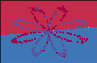
# Build a model with a n_h-dimensional hidden layer
parameters = nn_model(X, Y, n_h = 4, num_iterations = 10000, print_cost=True)

# Plot the decision boundary
plot_decision_boundary(lambda x: predict(parameters, x.T), X, Y)
plt.title("Decision Boundary for hidden layer size " + str(4))

# Print accuracy
predictions = predict(parameters, X)
print ('Accuracy: %d' % float((np.dot(Y,predictions.T) + np.dot(1-Y,1-predictions.T))/float(Y.size)*100) + '%')
Cost after iteration 0: 1.127380
Cost after iteration 1000: 0.288553
Cost after iteration 2000: 0.276386
Cost after iteration 3000: 0.268077
Cost after iteration 4000: 0.263069
Cost after iteration 5000: 0.259617
Cost after iteration 6000: 0.257070
Cost after iteration 7000: 0.255105
Cost after iteration 8000: 0.253534
Cost after iteration 9000: 0.252245
Accuracy: 91%

观测不同的隐藏层数对于模型的影响

1
2
3
4
5
6
7
8
9
10
11
12
# This may take about 2 minutes to run

plt.figure(figsize=(16, 32))
hidden_layer_sizes = [1, 2, 3, 4, 5, 20, 50]
for i, n_h in enumerate(hidden_layer_sizes):
plt.subplot(5, 2, i+1)
plt.title('Hidden Layer of size %d' % n_h)
parameters = nn_model(X, Y, n_h, num_iterations = 5000)
plot_decision_boundary(lambda x: predict(parameters, x.T), X, Y)
predictions = predict(parameters, X)
accuracy = float((np.dot(Y,predictions.T) + np.dot(1-Y,1-predictions.T))/float(Y.size)*100)
print ("Accuracy for {} hidden units: {} %".format(n_h, accuracy))
Accuracy for 1 hidden units: 61.5 %
Accuracy for 2 hidden units: 70.5 %
Accuracy for 3 hidden units: 66.25 %
Accuracy for 4 hidden units: 90.75 %
Accuracy for 5 hidden units: 90.5 %
Accuracy for 20 hidden units: 92.0 %
Accuracy for 50 hidden units: 90.75 %