本文主要参考自吴恩达Coursera深度学习课程 DeepLearning.ai 编程作业(1-4)
吴恩达Coursera课程 DeepLearning.ai 编程作业系列,本文为《神经网络与深度学习》部分的第四周“深层神经网络”的课程作业。
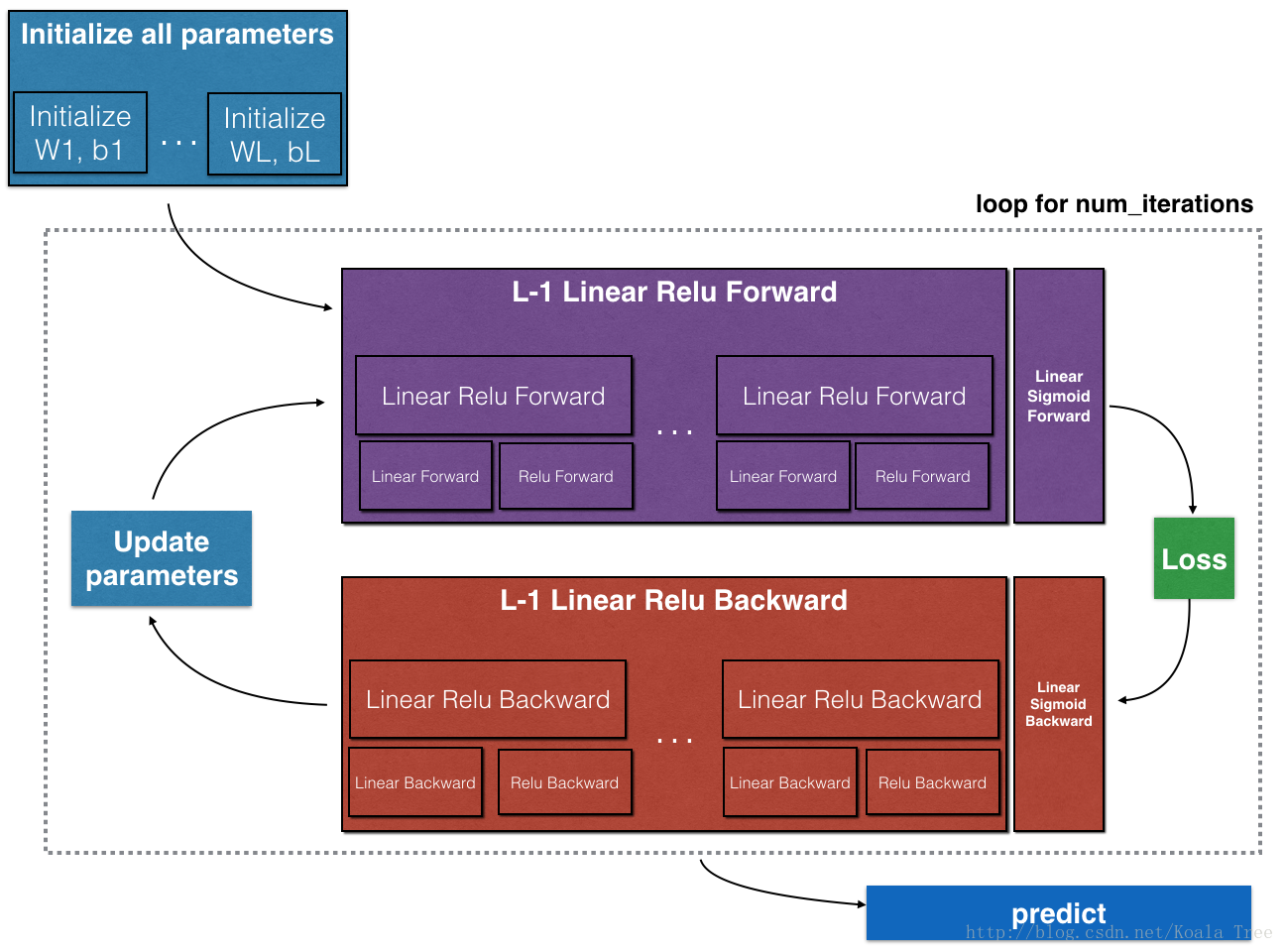
本节的主要内容是:实现L层的神经网络
大纲
首先完成一些helper function。然后再建立两层、多层神经网络:
- 两层和多层神经网络的初始化
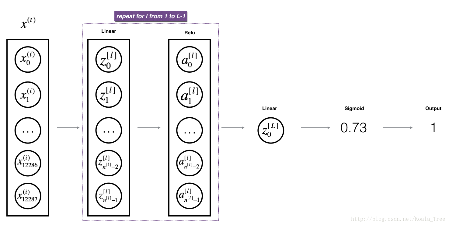
- 实现前向传播模型
- 实现某一层的前向传播 - 输出\(Z^{[l]}\)
- 激活层已给出
- 将前两步结合
- 将前向传播迭代L-1次,然后将激活层加到最后,就完成了L层的前向传播
- 计算误差
- 实现后向传播模型
- 实现某一层的后向传播
- 激活层的后向传播已给出
- 将前两步结合
- 将后向传播迭代L-1次,然后将激活层加到最后,完成了L层的后向传播
- 更新参数
import
1 | import warnings |
初始化
- 完成两层模型的初始化
- 完成多层模型的初始化
两层模型的初始化
- 模型结构是: LINEAR - RELU - LINEAR - SIGMOID
- 用随机数初始化w
- 用0初始化b
1 | # 参数初始化 |
W1 = [[ 0.01624345 -0.00611756 -0.00528172]
 [-0.01072969  0.00865408 -0.02301539]]
b1 = [[ 0.]
 [ 0.]]
W2 = [[ 0.01744812 -0.00761207]]
b2 = [[ 0.]]
L层模型的初始化
这个比较复杂。我们先来看一个X.shape = (12288,209)的例子:
| W.shape | b.shape | A | A.shape | |
|---|---|---|---|---|
| Layer 1 | (n[1],12288) | (n[1],1) | Z[1]=W[1]X+b[1] | (n[1],209) |
| Layer 2 | (n[2],n[1]) | (n[2],1) | Z[2]=W[2]A[1]+b[2] | (n[2],209) |
| ⋮ | ⋮ | ⋮ | ⋮ | ⋮ |
| Layer L-1 | (n[L−1],n[L−2]) | (n[L−1],1) | Z[L−1]=W[L−1]A[L−2]+b[L−1] | (n[L−1],209) |
| Layer L | (n[L],n[L−1]) | (n[L],1) | Z[L]=W[L]A[L−1]+b[L] | (n[L],209) |
实现: - 模型结构是 [LINEAR -> RELU] × (L-1) -> LINEAR -> SIGMOID . 也就是说,有L-1层的ReLU激活函数,还有一层sigmoid输出 - w用随机初始化 - b用0初始化 - 将\(n^{[l]}\)存入数组变量layer_dims中,代表第l层的n
1 | def initialize_parameters_deep(layer_dims): |
W1 = [[ 0.00319039 -0.0024937   0.01462108 -0.02060141 -0.00322417]
 [-0.00384054  0.01133769 -0.01099891 -0.00172428 -0.00877858]
 [ 0.00042214  0.00582815 -0.01100619  0.01144724  0.00901591]
 [ 0.00502494  0.00900856 -0.00683728 -0.0012289  -0.00935769]]
b1 = [[ 0.]
 [ 0.]
 [ 0.]
 [ 0.]]
W2 = [[-0.00267888  0.00530355 -0.00691661 -0.00396754]
 [-0.00687173 -0.00845206 -0.00671246 -0.00012665]
 [-0.0111731   0.00234416  0.01659802  0.00742044]]
b2 = [[ 0.]
 [ 0.]
 [ 0.]]
前向传播
按照如下顺序实现: - LINEAR - LINEAR -> ACTIVATION where ACTIVATION will be either ReLU or Sigmoid. - [LINEAR -> RELU] × (L-1) -> LINEAR -> SIGMOID (whole model)
LINEAR
线性模型如下:
\[Z^{[l]} = W^{[l]}A^{[l-1]} +b^{[l]}\tag{4}\]
where \(A^{[0]} = X\).
1 | def linear_forward(A,W,b): |
Z = [[ 3.26295337 -1.23429987]]
LINEAR -> ACTIVATION
本层的公式是:
\(A^{[l]} = g(Z^{[l]}) = g(W^{[l]}A^{[l-1]} +b^{[l]})\)
其中,g()有两种选择:
sigmod :
\(\sigma(Z) = \sigma(W A + b) = \frac{1}{ 1 + e^{-(W A + b)}}\)
sigmod的实现如下所示
输出: - A - cache = z
ReLU :
\(A = RELU(Z) = max(0, Z)\)
ReLU的实现如下所示 输出: - A - cache = Z
1 | def sigmoid(Z): |
1 | # 实现LINEAR->ACTIVATION层 |
With sigmoid: A = [[ 0.96890023  0.11013289]]
With ReLU: A = [[ 3.43896131  0.        ]]
L-Model Forward
- 用RELU,重复之前的linear_activation_forward,L-1次
- 最后输入SIGMOID 的linear_activation_forward
1 | def L_model_forward(X, parameters): |
X.shape = (4L, 2L) ,即 4 行 2 列
AL = [[ 0.17007265  0.2524272 ]]
Length of caches list = 2
计算误差
误差公式如下:
\[-\frac{1}{m} \sum\limits_{i = 1}^{m} (y^{(i)}\log\left(a^{[L] (i)}\right) + (1-y^{(i)})\log\left(1- a^{[L](i)}\right)) \tag{7}\]
1 | def compute_cost(AL, Y): |
cost = 0.414931599615
后向传播
后向传播是用来计算梯度的
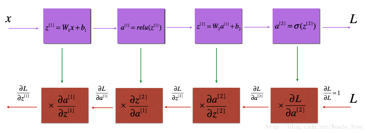
紫色方块代表前向传播 红色方块代表后向传播
我们的目标是计算出\(dw^{[l]}和db^{[l]}, l = 1,2,...L\),以便之后更新w和b。
为了计算\(dw^{[1]}和db^{[1]}\),要使用如下链式法则:
\(dw^{[1]}=\frac{dL}{dw^{[1]}}=\frac{dL}{dz^{[1]}} \times \frac{dz}{dw^{[1]}}=dz^{[1]}\times \frac{dz}{dw^{[1]}}\)
\(db^{[1]}=\frac{dL}{db^{[1]}} = \frac{dL}{dz^{[1]}} \times \frac{dz^{[1]}}{db^{[1]}} = dz^{[1]} \times \frac{dz^{[1]}}{db^{[1]}}\)
因此我们首先要算出\(dz^{[1]}\) :
\[\frac{dL(a^{[2]},y)}{dz^{[1]}}=\frac{dL(a^{[2]},y)}{da^{[2]}}\frac{da^{[2]}}{dz^{[2]}}\frac{dz^{[2]}}{da^{[1]}}\frac{da^{[1]}}{dz^{[1]}}\]
而要算出\(dz^{[1]}\),由上公示可以看出,我们必须先计算\(dz^{[2]}\)等
因此此过程叫做后向传播
总之,后向传播需要完成: - LINEAR - LINEAR -> ACTIVATION - [LINEAR -> RELU] × (L-1) -> LINEAR -> SIGMOID backward (whole model)
LINEAR
对于第l层来说,这一层的Linear部分是:\(Z^{[l]} = W^{[l]} A^{[l-1]} + b^{[l]}\)
假设此时你已经计算好了 \(dZ^{[l]} = \frac{\partial \mathcal{L} }{\partial Z^{[l]}}\)
你接下来想要得到\((dW^{[l]}, db^{[l]} dA^{[l-1]})\)
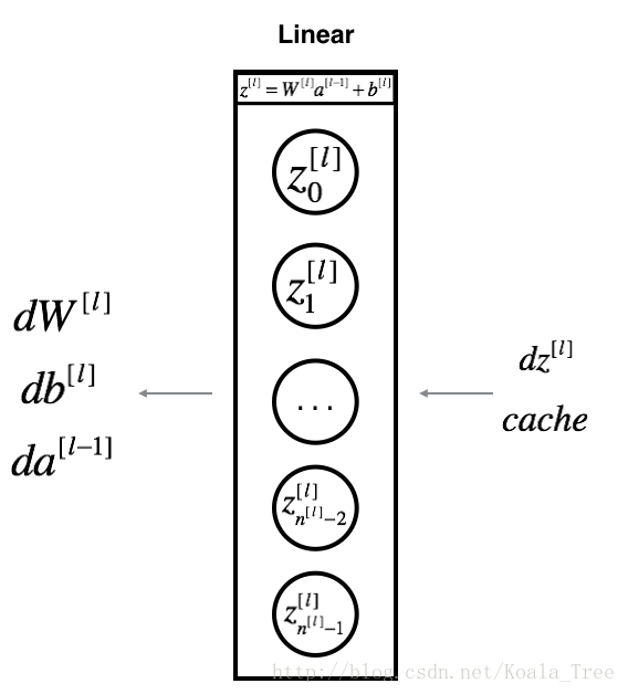
我们可以通过如下的公式,通过\(dZ^{[l]}\)来计算出这三个东西\((dW^{[l]}, db^{[l]}, dA^{[l-1]})\):
\[ dW^{[l]} = \frac{\partial \mathcal{L} }{\partial W^{[l]}} = \frac{1}{m} dZ^{[l]} A^{[l-1] T} \tag{8}\] \[ db^{[l]} = \frac{\partial \mathcal{L} }{\partial b^{[l]}} = \frac{1}{m} \sum_{i = 1}^{m} dZ^{[l](i)}\tag{9}\] \[ dA^{[l-1]} = \frac{\partial \mathcal{L} }{\partial A^{[l-1]}} = W^{[l] T} dZ^{[l]} \tag{10}\]
1 | def linear_backward(dZ, cache): |
dA_prev = [[ 0.51822968 -0.19517421]
 [-0.40506361  0.15255393]
 [ 2.37496825 -0.89445391]]
dW = [[-0.10076895  1.40685096  1.64992505]]
db = [[ 0.50629448]]
LINEAR -> ACTIVATION
本节要加入后向传播中的activation部分:
假设\(g(.)\)是激活函数,
而下面给出的两个函数:sigmoid_backward 和 relu_backward 计算了\(dL/dz\) : \[dZ^{[l]} = dA^{[l]} * g'(Z^{[l]}) \tag{11}\].
1 | def relu_backward(dA, cache): |
1 | def linear_activation_backward(dA, cache, activation): |
sigmoid:
dA_prev = [[ 0.11017994  0.01105339]
 [ 0.09466817  0.00949723]
 [-0.05743092 -0.00576154]]
dW = [[ 0.10266786  0.09778551 -0.01968084]]
db = [[-0.05729622]]

(1L, 2L)
(1L, 2L)
relu:
dA_prev = [[ 0.44090989 -0.        ]
 [ 0.37883606 -0.        ]
 [-0.2298228   0.        ]]
dW = [[ 0.44513824  0.37371418 -0.10478989]]
db = [[-0.20837892]]
L-Model Backward
接下来就该将后向传播应用在整个网络了。步骤如下:
- 前向传播 -
L_model_forward(),在每一层都存下了(X,W,b,z) - 后向传播 -
L_model_backward(),利用之前存的值,一层层向前计算导数
后向传播计算导数的流程如下图所示: 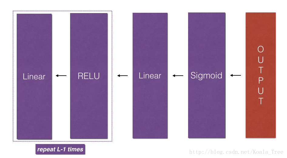
初始化部分
对于贯穿网络的后向传播来说,我们知道输出是\(A^{[L]} = \sigma(Z^{[L]})\). 我们需要计算出 : dAL \(= \frac{\partial \mathcal{L}}{\partial A^{[L]}}\).
为了完成这个目标,我们用如下公式实现: 1
dAL = - (np.divide(Y, AL) - np.divide(1 - Y, 1 - AL)) # 相对于AL的成本衍生物
接下来就该计算LINEAR->RELU后向传播部分了,这一部分需要存储每一步的dA, dW, db,用如下公式实现: \[grads["dW" + str(l)] = dW^{[l]}\tag{15} \] 例如,l=3,就将dw3 存储在grads["dw3"]中
1 | def L_model_backward(AL, Y, chache): |
(3L, 2L)
(3L, 2L)
dW1 = [[ 0.41010002  0.07807203  0.13798444  0.10502167]
 [ 0.          0.          0.          0.        ]
 [ 0.05283652  0.01005865  0.01777766  0.0135308 ]]
db1 = [[-0.22007063]
 [ 0.        ]
 [-0.02835349]]
dA1 = [[ 0.          0.52257901]
 [ 0.         -0.3269206 ]
 [ 0.         -0.32070404]
 [ 0.         -0.74079187]]
更新参数
在这一部分我们用以上模型更新参数:
\[ W^{[l]} = W^{[l]} - \alpha \text{ } dW^{[l]} \tag{16}\] \[ b^{[l]} = b^{[l]} - \alpha \text{ } db^{[l]} \tag{17}\]
其中,\(\alpha\)是学习率。
1 | def update_parameters(parameters, grads, learning_rate): |
W1 = [[-0.59562069 -0.09991781 -2.14584584  1.82662008]
 [-1.76569676 -0.80627147  0.51115557 -1.18258802]
 [-1.0535704  -0.86128581  0.68284052  2.20374577]]
b1 = [[-0.04659241]
 [-1.28888275]
 [ 0.53405496]]
W2 = [[-0.55569196  0.0354055   1.32964895]]
b2 = [[-0.84610769]]