LU分解条件
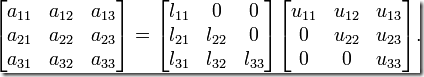
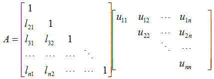
如果n阶方阵A的各阶顺序主子式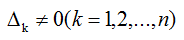 ,即A的各阶顺序主子矩阵Ak都可逆,则存在唯一的单位下三角矩阵L与唯一的非奇异上三角矩阵U,使得A=LU
其中k阶顺序主子式指 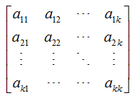
LU分解方法
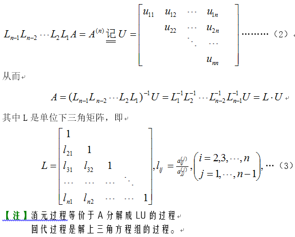
由于L存在可逆矩阵L',即LL'=E 则L'A=LL'U=U 因此得出一般的分解方法: 通过对(A,E)做初等行变换得到(U,L'),再由L'得到L.
其中:
- L是单位下三角矩阵(对角线上的系数都为1的下三角矩阵);L'也是单位上三角矩阵;
- U是非奇异上三角矩阵;
求解方法
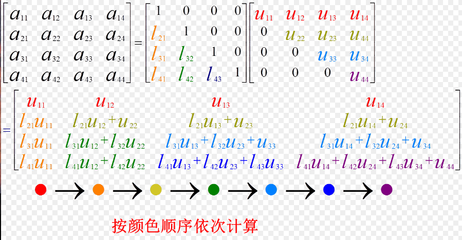
对于一般的线性方程组: \[Ax=b\] 如果我们能将A分解成\(A=LU\),即一个下三角阵和一个上三角阵U的乘积,那原方程组的解x便可由下面两步得到:
- 用前代法解\(Ly=b\)的y;
- 用回代法解\(Ux=y\)的x.

对于列主元消去法,求线性方程组\(Ax=b\)的计算过程可以按照以下步骤进行:
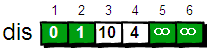
- 求A的列主元LU分解\(PA=LU\)
- 解下三角形方程组\(Ly=Pb\)
- 解上三角形方程组\(Ux=y\)
实现
前代法: 需要注意的是,回代法在计算的过程中需要考虑到主元位置序列,并同时对b进行调整。
double * forwardSub(double *lu,int n,double *b,int *p){
    //double *y=new double[n];
    double temp;
      //按qivot对b行变换,与LU匹配
      for(int i=0; i<n-1; i++)
      {
            temp = b[p[i]];
            b[p[i]] = b[i];
            b[i]=temp;
      }
    for(int i=0; i<n; i++)
            for(int j=0; j<i; j++)
                b[i]=b[i]-lu[n*i+j]*b[j];
    b[n-1]=b[n-1];
    return b;
}
回代法: 由于U是上三角矩阵,所以要从x[n-1]开始计算。
double * backSub(double *b,double *lu,int n){
     for(int i=n-1; i>=0; i--)
      {
            for(int j=n-1; j>i; j--)
                b[i]=b[i]-lu[n*i+j]*b[j];
            b[i]=b[i]/lu[n*i+i];
      }
    return b;
}
计算:
bool guass(double *lu,int *p,double*b,int n){
    double * y = forwardSub(lu,n,b,p);
    double * x = backSub(y,lu,n);
    std::cout<<endl<<"the sulution is ; "<<endl;
    for(int i=0;i<n;i++){
        std::cout<<x[i]<<"\t";
    }
    std::cout<<endl;
}
输出: 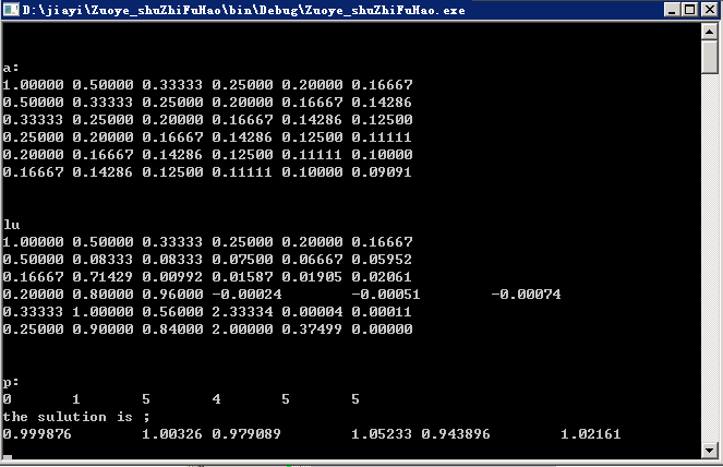
代码:
#include <iostream>
#include<cstdio>
#include<cstdlib>
#include<iomanip>
#define LIM -100000000
using namespace std;
double *luReult;
void printmat(double *mat,int n,string s){
std::cout<<endl<<endl<<s<<endl;
for(int i=0;i<n;i++){
for(int j=0;j<n;j++){
printf("%.5f\t",mat[i*n+j]);
}
std::cout<<endl;
}
}
void printarr(int *mat,int n,string s){
std::cout<<endl<<endl<<s<<endl;
for(int i=0;i<n;i++){
std::cout<<mat[i]<<"\t";
//printf("%s\t",mat[i]);
}
}
int findMainNumber(double *a,int n,int r){
float maxa=-99999;
int maxaIdx=-1;
//printmat(a,n,"a is now :");
for(int i=r;i<n;i++){
if(a[i*n+r]>maxa){
maxa=a[i*n+r];
maxaIdx=i;
}
}
return maxaIdx;
}
void exchange(double *a,int n,int e,int r){
float temp=0;
for(int i=0;i<n;i++){
temp = a[r*n+i];
a[r*n+i]=a[e*n+i];
a[e*n+i]=temp;
}
}
bool lu(double* a, int* pivot, int n)//矩阵LU分解
{
for(int k=0;k<n;k++){
//寻找第k列的主元
int p = findMainNumber(a,n,k);
exchange(a,n,p,k);//交换k行和p行
pivot[k]=p;//记录置换矩阵p
if(a[k*n+k]!=0){
for(int i=k+1;i<n;i++){//部分下三角L
a[i*n+k]=a[i*n+k]/a[k*n+k];
}
for(int i=k+1;i<n;i++){//计算上三角U
for(int j=k+1;j<n;j++){
a[i*n+j]=a[i*n+j]-a[i*n+k]*a[k*n+j];
}
}
}else{
return true;//矩阵奇异
}
}
/*
//计算下三角L
double temp=0;
for(int i=0; i<n-2; i++)//i行k列
for(int k=i+1; k<n-1;k++)
{
temp=a[n*pivot[k] + i];
a[n*pivot[k] + i]=a[k*n + i];
a[k*n + i]=temp;
}
*/
luReult=a;
printmat(a,n,"lu");
return false ;
}
double radio(int a,int b){
return (double)(a)/(double)(b);
}
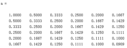
void buildHilbert(double *a,double *b,int n){
for(int r=0;r<n;r++){
for(int j=0;j<n;j++){
a[r*n+j]=radio(1,j+r+1);
b[r]=b[r]+a[r*n+j];
}
}
}
void exchangeb(double *b,int n,int r,int e){
double temp=0;
temp=b[e];
b[e]=b[r];
b[r]=temp;
/*r(int i=0;i<n;i++){
temp=b[r*n+i];
b[r*n+i]=b[e*n+i];
b[e*n+i]=temp;
}*/
}
double * forwardSub(double *lu,int n,double *b,int *p){
//double *y=new double[n];
double temp;
//按qivot对b行变换,与LU匹配
for(int i=0; i<n-1; i++)
{
temp = b[p[i]];
b[p[i]] = b[i];
b[i]=temp;
}
for(int i=0; i<n; i++)
for(int j=0; j<i; j++)
b[i]=b[i]-lu[n*i+j]*b[j];
b[n-1]=b[n-1];
return b;
}
double * backSub(double *b,double *lu,int n){
for(int i=n-1; i>=0; i--)
{
for(int j=n-1; j>i; j--)
b[i]=b[i]-lu[n*i+j]*b[j];
b[i]=b[i]/lu[n*i+i];
}
return b;
}
bool guass(double *lu,int *p,double*b,int n){
double * y = forwardSub(lu,n,b,p);
double * x = backSub(y,lu,n);
std::cout<<endl<<"the sulution is ; "<<endl;
for(int i=0;i<n;i++){
std::cout<<x[i]<<"\t";
}
std::cout<<endl;
}
int main()
{
int n=6;//矩阵是n*n的
double *b=new double[n];
double *a=new double[n*n];
/*double input[n*n]={0.001,1.00,1.00,2.00};
a=input;
double inputb[n]={1.00,3.00};
b=inputb;*/
buildHilbert(a,b,n);
printmat(a,n,"a:");
int *pivot=new int[n*n];
luReult=new double[n*n];
lu(a,pivot,n);
printarr(pivot,n,"p:");
guass(luReult,pivot,b,n);
//cout << "Hello world!" << endl;
return 0;
}
 ,则A有QR分解:
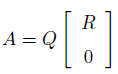 Q是mm的正交矩阵 R是nn的有非负对角元的上三角阵
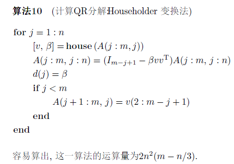
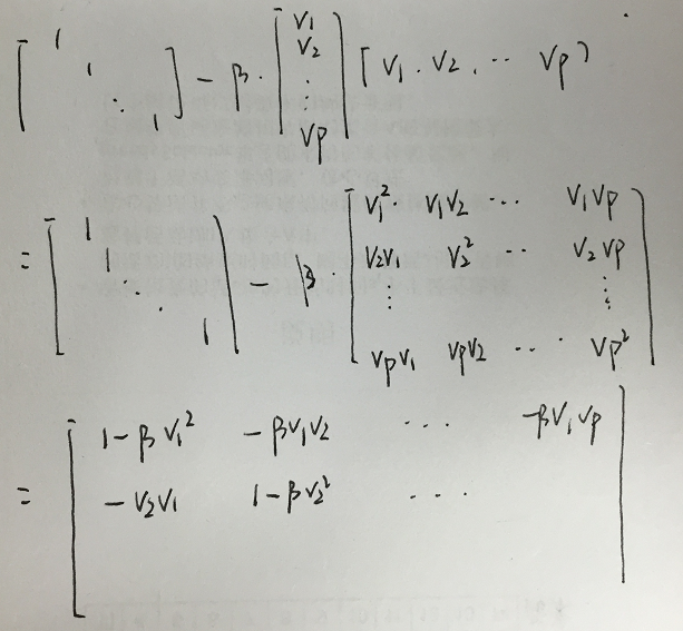
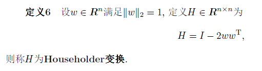

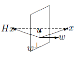
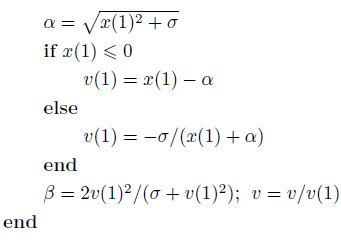
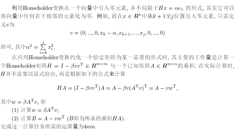
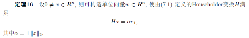 由以上定理可知,对于任意的x,都可以构造出Householder矩阵H,使得Hx的后n-1个分量为零。
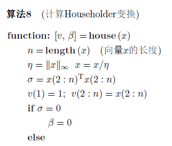
 其中,
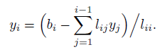
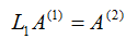
其中, 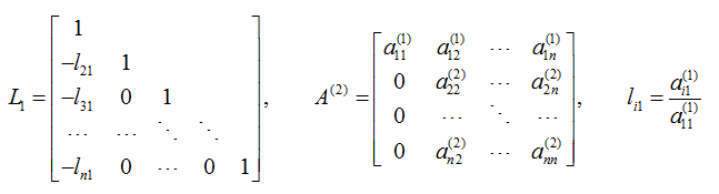 我们注意到li1恰好使得第i行的第一列元素变为零,即ai1-li1*a11=0。
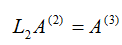
 其中,
其中,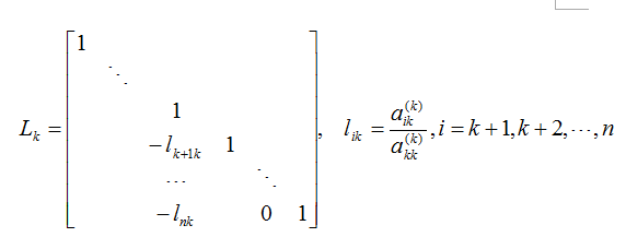
 初始(第一步):
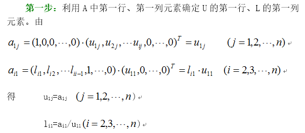

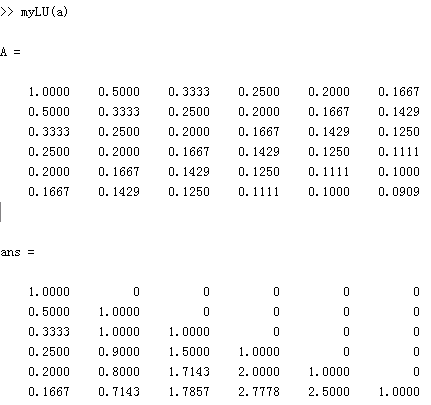 与我自己的L矩阵一致。决定还是相信自己。